When Artificial Intelligence learns from physics

Model-informed neural networks for describing wear phenomena

In recent years, Artificial Intelligence has become synonymous with automatic prediction: large amounts of data are fed into a neural network, which learns to reproduce a phenomenon. But is this really the best way to model a complex engineering system?
If we were to ask a linguist from the Accademia della Crusca to write a treatise on gravitational waves, they would probably have perfect knowledge of grammar and linguistic structure — but that does not mean they could automatically produce a scientific contribution on general relativity. In the same way, a neural network knows the statistical regularities of data, but it does not know the physics of the phenomenon it describes.
Artificial Intelligence does not replace the modeler; rather, it becomes a tool in their hands.

AI as a tool for physical modeling

At the Department of Industrial Engineering, we recently applied this approach to the study of emissions from automotive brake wear. The problem is complex: emissions depend on dissipated energy, deceleration, the history of previous braking events (bedding), and the evolution of the material’s surface state.
A purely data-driven approach might use a “generic” neural network, with many layers and thousands of parameters, leaving it to discover all relationships on its own.
But this has three well-known problems:

• Overfitting: the network learns the dataset but struggles to generalize.
• Lack of causal relationships: it learns correlations, not necessarily physical relations.
• Requirement for enormous amounts of data: this is the price of the model’s lack of physical knowledge.

If the network knows nothing about physics, it must “buy” knowledge with data.

Model-informed neural networks: giving structure to the network

The alternative is an approach we could call a model-informed neural network: a neural network whose structure is designed by the modeler based on knowledge of the physical phenomenon.
In the case of brake emissions, the model was built by separating two fundamental components:

1. A stationary part, a function of dissipated energy and deceleration.
2. A dynamic part, represented by an internal state that evolves over time and captures the system’s memory.

It is important to emphasize that in both parts the internal organization of the network is not arbitrary, but itself depends on specific knowledge of the physical phenomenon. The modeler decides which quantities are causally relevant, which are secondary, and for which component of the model they matter.
Not all variables play the same role: some quantities determine the stationary component (for example, dissipated energy); others influence the dynamics and memory of the system; still others can be treated as unmodeled noise.
In this sense, the modeler makes causal relationships explicit, specifies which quantities matter and for what they matter, and translates this knowledge into the very structure of the network.
This operation is equivalent to a process of expert-guided meta-learning: it is not only the network that learns from data, but the modeler who provides the network with a structure consistent with physics, restricting the space of possible solutions even before training.
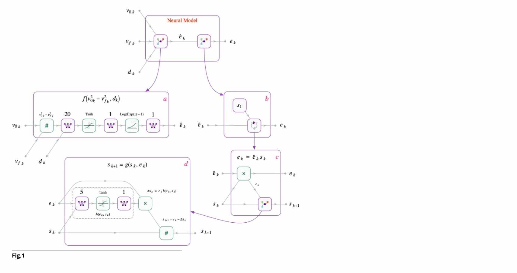
The resulting architecture is not an indistinct “black box”: a first module computes the baseline emission component; a second recurrent module updates an internal state that modulates emissions as a function of prior history.
The result is a model with just over one hundred parameters, but with a structure consistent with the physics of the problem.

Why is this approach powerful?

Computational efficiency.
The structure incorporates physical constraints, reducing parameters and the risk of overfitting.

Flexibility compared to rigid equations.
It allows complex nonlinearities to be modeled without formulating closed-form equations for each mechanism.

Integration between theory and experimentation.
It combines precise physical principles with rules learned from data.

A paradigm shift

The neural network is a sophisticated tool. Physics is the compass.
It is from the meeting of the two that a new frontier in the modeling of complex engineering systems emerges.

Fig.: Block diagram of the recurrent neural network model, composed of one module (a) that learns the function in (2) and a second module (b) that learns the state dynamics (3). Both modules have physics-informed structures.